
Heuristic optimization in classification atoms in molecules using GCN via uniform simulated annealing

In our research, we focus on developing a system for correctly classifying atoms in molecules based on input in the form of a graph, in which atoms are represented as vertices and chemical bonds are represented as edges. The goal of our system is to assign appropriate labels to atoms by using Graph Convolutional Network with residual connection. In addition, another optimization technique, the metaheuristic technique is introduced to better optimize and find the best parameters (weights).
Data preprocessing
Preparing the data for our GCN model was based on transforming the Coulomb matrix C for each molecule into corresponding neighborhood matrices A and node feature matrices X, as input to the graph network. First, in order to correctly create the adjacency matrix A, which determines the connections (chemical bonds) between atoms in the molecule, it was first identified whether the values of \(C_{ij}\) exceed a threshold of 2.1. Such a threshold value was taken to perform a preliminary selection of pairs of atoms for which the electrostatic interaction is strong enough to be treated as a potential chemical bond in the molecule. If the value of \(C_{ij} > 2.1\) we calculate a new value of \(C_{ij}^{‘}\) based on the atomic number \(Z_i\) and \(Z_j\) and the assumed characteristic bond length d between a particular pair of atoms. The threshold = 2.1 value was set as a preliminary acceptable level to minimize computational complexity and compare only those pairs of atoms for which the interaction values are greater than 2.1. For small values of the electrostatic interaction (below 2.1), the distances between pairs of atoms are too large to form a strong chemical bond. In this way, only those pairs for which the values of the Coulomb matrix C exceed the value of 2.1 will be checked. In our dataset, we distinguish only 5 classes of atoms such as: H, C, N, O and S and such a threshold value is safe and at the beginning of the process we can eliminate those pairs that will certainly not form a chemical bond. For a pair of C-H atoms, only a single bond can occur and its average length which we use in the calculations \(C_{ij}’\) is 1.09 Å, while the value of the electrostatic interaction \(C_{ij}’\) is 2.91 in atomic units. This is the lowest value that can appear in the Coulomb matrix \(C’\) for our database, because their atomic charge product is the lowest, because the overall bond lengths between atoms are approximate values in the range of 1-2Å, atomic numbers play a key role here, because they have a larger range. We do not consider H-H bonds, because they do not occur in complex molecules. This bond does not contribute to the stability of larger structures, and hydrogen prefers to combine with carbon, oxygen, or nitrogen. Additionally, the established bond length may change slightly depending on the chemical environment, external factors, hybridization, so they can be lengthened or shortened by very small values32. Therefore, the choice of threshold = 2.1 is a good and optimal approach, because for this measure we remove pairs of atoms for which interactions are too weak, thus eliminating unnecessary comparisons of new values of \(C_{ij}’\) with \(C_{ij}\). Moreover, the value 2.1 is much lower than the lowest value we can obtain when defining an interaction between a pair of C-H atoms. The determination of the new value of \(C_{ij}^{‘}\) is expressed as:
$$\begin{aligned} C_{ij}^{‘} = \frac{Z_i \cdot Z_j}{d \cdot k} \end{aligned}$$
(4)
where: d is the assumed bond length for a pair of atoms \({i-j}\) (e.g. \(d = 1.09 \,\)Å for a carbon-hydrogen bond). Additionally, a conversion factor k = 1.88973 was used to convert units from angstroms to atomic (Bohr) units. At the very end, to determine whether a pair of atoms forms a chemical bond, we check the difference between the new Coulomb value \(C_{ij}^{‘}\) and its initial value \(C_{ij}\) including a tolerance of 2.8:
$$\begin{aligned} |C_{ij}’ – C_{ij}| < tolerance \end{aligned}$$
(5)
If the given condition is met, we can conclude that there is a chemical bond (connection) between the atoms and the element of the adjacency matrix \(A_{ij}\) takes the value 1. The tolerance value is 2.8 to account for differences that may occur since we use average bond length values to calculate new Coulomb values. Furthermore, there may be different types of bonds between some pairs of atoms such as single, double and triple bonds, which have different average bond lengths. In this case, in our algorithm that calculates a new Coulomb value based on a pair of atoms that may have a single, double or triple bond, we first calculate the average value \(avg \ bond \ length\) based on three bond length values, similar to a carbon-oxygen pair, for which three bonds may occur, according to the formula:
$$\begin{aligned} {avg\ bond\ length} = \frac{d_{\beta – \gamma } + d_{\beta =\gamma } + d_{{\beta \equiv \gamma }}}{3} \end{aligned}$$
(6)
where: \(\beta\) and \(\gamma\) are two different atoms, \(d_{\beta – \gamma }\) – single bond, \(d_{\beta =\gamma }\) – double bond i \(d_{\beta \equiv \gamma }\) – triple bond. The tolerance condition is equal to 2.8 because this value takes into account all acceptable cases of deviations from the correct \(C_{ij}\) values, for all pairs of atoms. To sum up, our adjacency matrix preparation for the GCN model was based on 3 key steps. For each molecule, the Coulomb matrix was transformed into a neighborhood matrix by first checking the value with the threshold value, then calculating the new value and verifying it with the tolerance value. In addition, the X feature matrix for each molecule was constructed based on the \(C_{ii}\) diagonal elements of the Coulomb matrix corresponding to that molecule, and this matrix is represented as a vector:
$$\begin{aligned} {X} = [{C}_{11}, {C}_{22}, \dots , {C}_{NN}] \end{aligned}$$
(7)
In order to process many molecules simultaneously and reduce the calculation from the assumption that each molecule is represented by its quadratic adjacency matrix, we combined all the neighborhood matrices separately for the entire dataset (this process was done twice separately for the training and test data) consisting of J molecules into one large diagonal block matrix expressed by formula:
$$\begin{aligned} B = \begin{pmatrix} A^{(1)} & 0 & \cdots & 0 \\ 0 & A^{(2)} & \cdots & 0 \\ \vdots & \vdots & \ddots & \vdots \\ 0 & 0 & \cdots & A^{(J)} \end{pmatrix} \end{aligned}$$
(8)
In a similar way, one long resulting feature vector was created that combines the features of the atoms of all particles:
$$\begin{aligned} F = \begin{pmatrix} X^{(1)} \\ X^{(2)} \\ \vdots \\ X^{(N)} \end{pmatrix} \end{aligned}$$
(9)
where: \(X^{(p)}\) is the feature vector for p-th molecule. The data constructed in this way was used in the node classification problem considering only the adjacency matrices of all molecules and the corresponding feature vectors representing the properties of the nodes. In our research, we investigated how GCN with residual connection can analyze and aggregate information from neighbors which translates into efficient assignment of labels to unknown atoms based only on neighborhood information and their chemical properties.
GCN with residual connection
In this paper, we used Graph Convolutional Network13 with residual connection as an artificial intelligence model that efficiently classifies atoms (nodes) in graphs (molecules). Edges represent the relationship between individual nodes, which denote chemical bonds. GCNs are a type of neural networks that allow the study of complex and irregular structures. CNNs use filters that change the value of a pixel based on the surrounding pixels in the image, similarly, GCNs use the idea of convolution and update the value of a node by aggregating the features of the node’s neighbors. The main elements used in a graph layer are the adjacency matrix A of the graph \(G = (V,E)\) and the feature matrix X, which contains the features assigned to each node in the graph. In each graph layer there is a propagation process which is characterized by updating the features of all vertices in the graph, this process is denoted by the formula:
$$\begin{aligned} H^{(l+1)} = \sigma \left( \hat{D}^{-\frac{1}{2}} \hat{A} \hat{D}^{-\frac{1}{2}} H^{(l)} W^{(l)} \right) \end{aligned}$$
(10)
where: \(H^{(l)}\) denotes the features of the vertices in the l-th layer, \(H^{(l+1)}\) is the result of operations in the l-th layer, which will be used as input to the next layer. In addition, \(\hat{A}\) symbolizes a normalized neighborhood matrix described as \(A+I_N,\) where \(I_N\) is a identity matrix. Diagonal matrix \(\hat{D},\) where element \(\hat{D_{ii}}\) is the sum of values in the i-th row of matrix \(\hat{A}\). \(W^{(l)}\) is the weight matrix for the l-th layer which is trained during the training process and \(\sigma\) is the activation function (ReLU). Our model architecture consists of three graph layers: two graph layers with residual connection and the last layer terminated by a sigmoid or softmax activation function depending on the type of classification. The schematic of our entire model for the imbalanced dataset is presented in Fig. 2.

A schematic of the GCN model with residual connection for an unbalanced set for a single molecule is presented. The input to the system is a graph (molecule) \(G=(V,E)\) without assigned atom types. There are two graph Hidden Layers, which means two graph layers with our residual connection. In these layers, there is a process of extending the initial features of the graph from 1 to 32, and in each layer there is an aggregation of information from neighbors, and the process of updating the features of the nodes itself is completed by the activation function \(\sigma\) = ReLU. At the very end, there is a classic graph layer, which is terminated with another activation function \(\sigma =\)Softmax, since in our study, multi-class classification is performed for an imbalanced data set.
An extension of the classical graph layer used 2 times in our system was the introduction of the concept of residual connection, in a different way than was presented in the article13. The researchers proposed a method for feature propagation taking into account the residual connection after executing the activation function \(\sigma,\) in our graph layer the residual connection is added before the activation function \(\sigma,\) expressed by the formula:
$$\begin{aligned} H^{(l+1)} = \sigma \left( \hat{D}^{-\frac{1}{2}} \hat{A} \hat{D}^{-\frac{1}{2}} H^{(l)} W^{(l)} + H^{(l)} \right) \end{aligned}$$
(11)
In addition, we adopted the following dimensions of weights in order to extend the initial features of the nodes \(H^{(1)} \in \mathbb {R}^{N \times 1}\) to dimension 32 and to capture the complex relationships in the graph: the first layer contains \(W^{(1)} \in \mathbb {R}^{1 \times 32},\) the second layer \(W^{(2)} \in \mathbb {R}^{32 \times 32}\) and the third \(W^{(3)} \in \mathbb {R}^{32 \times c},\) where \(c=1\) for binary classification or \(c=4\) for multi-class classification. The output of our model is the classification of nodes (atoms) based on features and relationships in the graph as shown in Fig. 2. In our GCN model, where the input data have been combined, Eqs. 10 and 11 take the following forms:
$$\begin{aligned} F^{(l+1)} = \sigma \left( \hat{D}^{-\frac{1}{2}} \hat{B} \hat{D}^{-\frac{1}{2}} F^{(l)} W^{(l)} \right) \end{aligned}$$
(12)
$$\begin{aligned} F^{(l+1)} = \sigma \left( \hat{D}^{-\frac{1}{2}} \hat{B} \hat{D}^{-\frac{1}{2}} F^{(l)} W^{(l)} + F^{(l)} \right) \end{aligned}$$
(13)
So in our case, using the concept of residual connections is a good idea, because the features representing the nodes in the graph come from the Coulomb matrix (Eq.6). This allows us to distinguish different atoms and their influence on the environment. The GCN layers mainly work on updating the target node by propagating information from its neighbors, so the new representation of a given atom is updated based on the features of its neighbors. After a few GCN layers, the model will distinguish the influence of neighboring atoms, naturally distinguishing that the presence of oxygen affects differently than the presence of hydrogen without using additional attention mechanisms for connections as in GAT33.The aforementioned GAT introduces a dynamically learned edge weights mechanism, which allows the model to decide which edges are more important than the rest. This approach is often used in situations where the connections between nodes are ambiguous or difficult to notice, and in our case the bonds between atoms were precisely defined by the chemical bonds formed between them, each of which is important and represents the real relationship between atoms in the given molecules. The use of the GAT mechanism would increase additional computational complexity, because it would require additional actions to calculate the attention for each edge in the graph, which would result in a longer training process. According to our experiments, our GCN model allowed for obtaining high prediction efficiency, so the attention mechanism itself would not significantly improve the quality of classification, only increasing the computational complexity. The use of other techniques such as transformers in graphs (Graph Transformer)34, taking into account attention mechanisms, positional encoding and the use of edge features, is not necessary for our problem. In the case of atom classification, only local information is important since nodes directly interact only with their neighbors, and using a long-distance mechanism would be inappropriate for atom prediction since several GCN layers allow access to further neighbors, so using a Graph Transformer would not provide additional benefit.
Uniform simulated annealing
The Simulated Annealing algorithm was first mentioned in35. This method resembles the phenomenon of annealing in metallurgy. Annealing is a popular heat treatment process used to change the physical and mechanical properties of a material to reduce their hardness, increase ductility and eliminate internal stresses. Annealing involves heating a metal or metal alloy object to a certain temperature, keeping it there for a certain period of time and then slowly cooling it down.

The operating procedure of the Simulated Annealing algorithm: blue dot – the initial solution, red dot – local minimum, green dot – global minimum and Hill Climbing – movement is accepted with a certain probability.
Boltzmann distribution is the essential key of this method, which determines the probability of a system held at temperature T being in an energy state E:
$$\begin{aligned} P(E) = \exp (-E/kT) \end{aligned}$$
(14)
where: k is Boltzmann constant. The main advantage of this iterative algorithm is that it can select an inferior solution with a certain probability. This is to get out of the local minimum and continue towards the optimal solution. The operation of the algorithm is shown in Fig.3, which shows Hill Climbing situations (selection of the second condition) when stuck in the local minimum. Thus, an important parameter is the temperature, the higher the temperature, the higher the probability of accepting a worse solution. The lower, the more the algorithm concentrates on local optimization. In our paper, we propose the Uniform SA algorithm to optimize the weights W in our graph network. The weights will be first optimized with metaheuristics, then optimized with gradient algorithms, in order to maximize the tuning of the weights. Our proposed USA (Uniform Simulated Annealing) algorithm includes the standard SA assumptions, which are: initialization of a random initial solution \(x_0\) (additionally, e.g. including setting initial parameters for temperature etc.), generation of a new solution by perturbation (small change) of the current solution, setting acceptance criteria based on the Metropolis equation, gradual cooling of the temperature and setting a stop condition. Due to the fact that our chosen perturbation using the uniform distribution from the range \([-b,b)\) was the best option in the context of weight optimization, our optimizer was given the ’Uniform’ prefix, emphasizing its subtype for this type of problem due to the type of distribution used in graph network optimization. We want to emphasize that we use the uniform distribution, and not other popular techniques such as the normal distribution, perturbation related to decreasing temperature, or as in the traveling salesman problem, where new solutions are obtained by swapping two random elements. The uniform distribution has an advantage over the popular normal distribution, because each value from a given range is equally probable, so it gives a chance for greater changes at the beginning of training, providing a larger space for exploring new, potentially better solutions (weights), which will then only be fine-tuned in the next stage of training (using the gradient approach).
The overall optimization will be subjected to a total of 3 layers of our network: \(W = \{W^{(1)},W^{(2)},W^{(3)}\},\) where each \(W^{(l)}\) denotes the weight matrix for the l-th layer in the model. In addition, we applied one more improvement, namely the addition of the number of neighbors, which allows the Uniform SA algorithm to search even more.
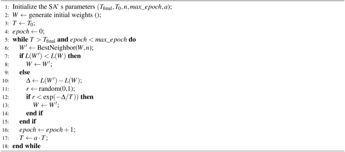
Uniform Simulated Annealing
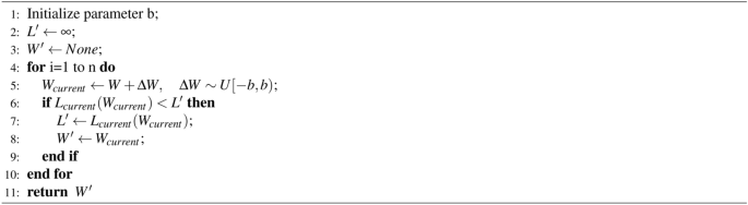
The operation of the USA algorithm is presented in pseudo-code. As function L, we defined the loss function used during training of the model. It is required to pre-initialize parameters such as \(T_{\text {final}},\) \(T_0,\) n (neighborhood size), \(max\_epoch,\) a. The generation of the initial solution W is done randomly. The new potential solution \(W’\) is generated using the function BestNeighbor, which creates new values based on a uniform distribution over the interval \([-b,b).\) Ultimately, the new solution is compared with the previously accepted one; if it is inferior it is accepted with a certain probability. The coefficient T, on the other hand, gradually decreases. In summary, the probability of adopting an inferior solution decreases as the temperature decreases and the difference in the loss of the two solutions increases. Our Uniform Simulated Annealing algorithm distinguishes the mechanism of generating n-perturbations in the BestNeighbor function, thus creating n-neighbors. The use of this function distinguishes the classical approach of the SA algorithm36, in which only one perturbation is created during one epoch. Additionally, in the modified SA algorithm, a new solution is generated in a fixed neighborhood size. In our concept, the process of selecting the best perturbation among all is based on its quality (cost function) of the modified weights, and the process itself promotes even broader exploration of solutions. The BestNeighbor algorithm is executed only once for each epoch and works as follows: n-neighbors are generated by adding small random values (perturbations) from the uniform distribution to the weights \(W^{(1)},\) \(W^{(2)}\) and \(W^{(3)},\) creating new values of weights:
$$\begin{aligned} \begin{aligned} W_i^{(1)} = {W_i}^{(1)} + \Delta W_i^{(1)} \quad \text {for} \quad i = 1, 2, \dots , n \\ W_i^{(2)} = {W_i}^{(2)} + \Delta W_i^{(2)} \quad \text {for} \quad i = 1, 2, \dots , n \\ W_i^{(3)} = {W_i}^{(3)} + \Delta W_i^{(3)} \quad \text {for} \quad i = 1, 2, \dots , n \end{aligned} \end{aligned}$$
(15)
where: \(\Delta W_i^{(1)} \in R^{1\times 32},\) \(\Delta W_i^{(2)} \in R^{32 \times 32},\) \(\Delta W_i^{(3)}\in R^{32\times c}\) are the perturbation matrices for n versions. Then, for each i-th version of weights, the model loss is calculated and the i-th version of weights is selected, for which the loss among n-neighbors is the lowest. Then, the best weight values are returned from the BestNeighbor function and the classic mechanism of accepting 1 or 2 conditions is followed. This approach allows for the selection of the best neighbor option, containing the smallest loss function. However, according to our experiments, this approach requires setting a slightly larger interval \([-b,b)\) due to the fact that the generated new solutions may always turn out to be better, tending from the beginning to the local minimum. A larger interval \([-b,b)\) allows for obtaining solutions from a larger space, avoiding a situation in which the sought solution will be in the local minimum from the beginning. Therefore, a larger interval allows us to be on the right track to the global minimum of our objective function. The value of b set by us is constant and does not change during the algorithm’s operation. In addition, an important parameter is the appropriate choice of the number of neighbors involved in generating new solutions. In order to select the best neighborhood size, we tested the performance of our Uniform SA algorithm for 4 different neighborhood sizes: 1, 5, 10 and 20. The results are presented in Fig.4.

Impact of Neighbors. Loss functions for different selection of neighbors in the Uniform Simulated Annealing algorithm. The largest number of neighbors led to the lowest loss function.
If fewer neighborhoods are chosen: 1 or 5, the algorithm runs faster but does not give better solutions, due to less exploration. In addition, it can more easily get stuck in local minima and hit solutions of poorer quality. The best results occur for the number of neighbors equal to 20. The resulting loss is the lowest, and the graph of the loss function is least susceptible to sudden upward jumps in the training process. In the SA technique with a higher number of neighbors, such as 10 and 20, there is a greater chance of accepting 1 conditions due to the large number of potential solutions generated during one epoch, which makes the loss function graphs smoother and smoother. In view of the experiment, a neighborhood size value of 20 was chosen for further testing.
Additionally, as shown in Fig. 4 for each number of neighbors the algorithm reaches a stable state of the loss value after 15 epochs. The best convergence is visible for n = 20 neighbors, the loss function does not jump, is reduced the fastest and stabilizes at the lowest level. Similarly, for the gradient method the loss function also decreases which means the weights are fine-tuned and after some time the loss value stabilizes again which means the final convergence of the model. In this way the gradients do not start with random weight values, but with values generated by the USA, therefore the decrease is even more effective. This means that our USA algorithm found favorable initial weights, which were later trained by the gradient optimizer. However, the computational complexity of the USA is slightly higher than in the classical SA algorithm due to the generation of n-perturbations per epoch and not just one random one. This approach has the advantage that we can choose such a solution from n-neighbors, which speeds up the convergence process, as shown in Fig. 4, where a larger number of neighbors supports even better convergence. The Uniform Simulated Annealing with the gradient optimizer is a combination of initial exploration and later exploitation. The values presented in Fig. 7 prove that the difference in the weight values after the USA algorithm and after the gradient optimizer are small, which indicates that the USA provides very good initial weights, which are then efficiently tuned.
Dataset
The QM7 Dataset37,38 was used to conduct the study. The set is a subset of GDB-13 consisting of molecules up to 23 atoms, including molecules consisting of atoms: H, C, N, O and S. In total, our QM7 dataset contains 7165 molecules. Examples of molecules created from the processed data in visual form are shown in Fig. 5.

Sample molecules from the QM7 Dataset.
For detailed optimization studies, we divided the collection into two bases: imbalanced and balanced. The imbalanced base contains molecules consisting of the four dominant atoms of H, C, N and O. Molecules containing sulfur atoms were omitted due to the small-volume collection of these atoms in the entire QM7 Dataset. The balanced base contains molecules we selected that contain only 2 classes: hydrogen and carbon atoms in proportions of 60 and 40. Based on the classification of the degree of class imbalance described in the39, this collection can be described as very close to equilibrium, since the percentage of the minor class is in the range (20–40%). The distribution of the two databases is shown in Tables 1 and 2.
link


.jpg "IFW Dresden selects Agnitron Agilis 100 MOCVD platform for precursor chemistry and ultra-wide-bandgap materials development")